Israeli elections on Twitter
By Amit Levinson in R
April 20, 2020
Introduction
Israel had its 3rd election within 12 months on March 2, 2020. This is because our Knesset - Hebrew term for house of representatives - wasn’t able to form or hold a government after each of the previous elections. As I won’t get into the politics of why they didn’t succeed in forming one (get it? politics 😉), I do want to take the opportunity and analyze some tweets posted in the time before and after the elections.
When we think of a data aggregating tweets, many questions arise - who, what, when, where and more about our data. Namely, with the collected data I want to answer the following questions:
- What was the frequency of tweets associated with the word ‘elections’?
- Who tweeted the most?
- What was the most common #Hashtag tweeted?
- Which tweet was most liked and which was retweeted the most?
- What were the most common words and bigrams (two words) in tweets?
Gathering the data
Twitter’s API allows scraping 6-9 days back for free. Therefore, I scraped the data already on March 7, 2020 and saved it for later use.
Let’s start with the packages we’ll use:
library(rtweet)
library(tidyverse)
library(tidytext)
library(igraph)
library(hrbrthemes)
library(ggraph)
library(extrafont)
I could use a consistent plot theme throughout the post but I’ll probably be editing each one a bit, while also some are not our regular graphs. With that said, There are some tweaks that will be consistent acorss several of the plots. Therefore, let’s create a theme function as a supplement to all other theme arguments I’ll use that will save a few lines of code:
mini_theme <- function(family = "Roboto Condensed", tsize = 16) {
  theme_classic() +
  theme(text = element_text(family = family),
        axis.ticks = element_blank(),
        axis.line = element_blank(),
        plot.title = element_text(size = tsize))}
Next we’ll gather the tweets we need:
elections_raw <- search_tweets("בחירות", n = 18000, retryonratelimit = TRUE)
To gather the tweets we can use the {rtweet} package which is amazing for collecting Twitter data. As I mentioned earlier, I already scraped the data a few days after the elections but left the command here to show what we did and how easy it is to do it. I searched only one term, ‘elections’ in Hebrew, and rtweet gathered all tweets containing that word.
What did our search yield? Let’s have a look:
dim(elections)
## [1] 16560 90
16,560 rows and 90 columns! As we can see, the {rtweet} package brings back a lot of information!
Some Caveats:
Before we begin, I will say this post doesn’t aim to be representative of the discussions that were held during the election period. As a matter of fact, nor does it aim to be representative of the twitter discussions surrounding the elections. this is due to two main reasons:
-
Twitter isn’t common in Israel at all. I’m not sure what’s the usage rate but it’s definitely not representative of the Israeli population.
-
I searched for only one word - elections (in Hebrew) - which yielded some 16560 tweets. This is definitely not a large enough pool of tweets to claim for representation.
With that said, the data gathered provides an opportunity to look at some Twitter data from the election period and motivate others to use the {rtweet} package, so why not give it a go.
Tweet frequency
First, let’s see how the tweets distribute across the time span we searched for. we can create a quick time plot using the ts_plot() argument from the {rtweet} package:
elections %>%
  ts_plot("2 hours")+
  geom_line(size = 1, color = "black")+
  mini_theme()+
  scale_x_datetime(date_breaks = "1 day",date_labels = "%d %b")+
  labs(x= NULL, y = NULL,
       title = "Tweet frequency throughout the Israeli elections week",
       subtitle = "Tweets aggregated by two-hour interval. Only tweets containing the word 'elections'\nin Hebrew were gathered")+
  geom_text(aes(x = as.POSIXct("2020-03-02 23:00:00"), y = 435, label = "10 PM:\nPolls close"),
            hjust = 0, size = 3, family = "Roboto Condensed")+
  geom_vline(xintercept = as.POSIXct("2020-03-02 22:00"),linetype = "dashed", size = 0.5, color = "black", alpha = 5/10)+
  theme(plot.subtitle = element_text(color = "gray70"))
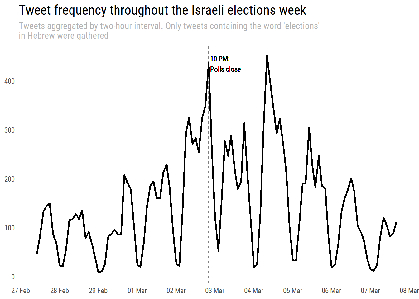
Interesting - we see the number of tweets during the closing time is equivalent to that of midday on March 4th. Most of the votes were counted by the end of March 3rd, so I can’t really put my finger on what this jump represents. After all, I collected tweets containing our word so it could have been that many people tweeted that specific term in that time slot. Anyway, I wasn’t able to find anything interesting that happened on the news that day but feel free to explore and offer suggestions.
Users with most tweets
Next, let’s look at who tweeted the most:
elections %>%
  count(screen_name, sort = T) %>%
  slice(1:15) %>%
  mutate(screen_name = reorder(screen_name,n)) %>%
  ggplot(aes(x= screen_name, y= n))+
  geom_col(fill = "gray70")+
  coord_flip()+
  scale_y_continuous(breaks = seq(0,180, 30), labels = seq(0,180,30))+
  labs(x = "Screen name", y = "Number of tweets", title = "Top 15 users tweeting the word 'elections'")+
  mini_theme()+
  theme(text = element_text(family = "Calibri"),
        axis.text = element_text(size = 12),
        axis.title.y = element_blank())
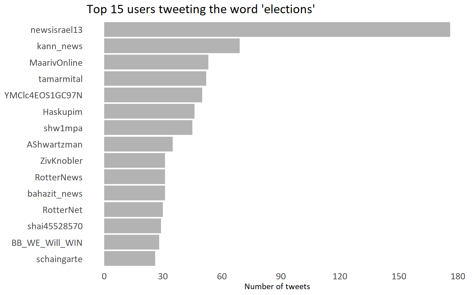
We see that many news companies tweeted a lot using the word ‘elections’: ‘newisrael13’, ‘kann_news’, ‘MaarivOnline’, ‘RotterNews’, ‘bahazit_news’, ‘RotterNet’. I personnaly don’t recognize the rest, but on the other hand I use Twitter mostly to follow R and academic related tweets, not necessarily Israeli politics.
Common Hashtags
When using the {rtweet} package to gather twitter data, one of the variables collected is the hashtags used in tweets. Although it doesn’t require too many lines of code to extract hashtags out of text, I think this is an amazing feature that shows the effort and details
Michael W. Kearney and contributors put into the package.
According to Wikipedia, a ‘Hashtag’ “is a type of metadata tag used on social networks such as Twitter and other microblogging services.”, that basically tags the message with a specific theme. This helps to see trends and themes in a macro level.
OK then, let’s see what we have:
hashtags <- elections %>%
  select(hashtags) %>%
  unlist() %>%
  as.tibble() %>%
  mutate(value = tolower(value)) %>%
  count(value, name = "Count", sort = T) %>%
  mutate(value = reorder(value, Count),
         iscorona = ifelse(value == "קורונה" | value == "coronavirus", "y", "n")) %>%
  filter(!is.na(value)) %>%
  slice(1:20)

ggplot(data = hashtags, aes(x = Count, y = value, fill = iscorona))+
  geom_col(show.legend = FALSE)+
  scale_fill_manual(values = c(y = "#1DA1F2", n = "gray70"))+
  labs(y = NULL, x = "Number of Tweets", title = "Top 20 Hashtags addressing the Israeli elections")+
  mini_theme()+
  theme(text = element_text(family = "Calibri"),
        axis.text = element_text(size = 12))
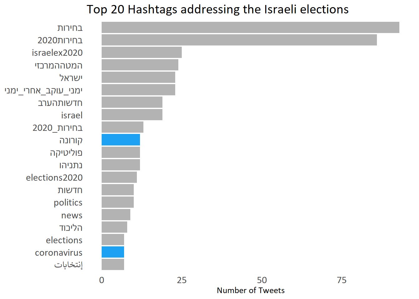
The tweets include pretty much what we expect - hashtags about the elections - with the two leading ones being ‘elections’ and ‘elections2020’. We also see a peculiar hashtag ‘right_following_right_people’, and others such as ‘Netanyahu’ (the Prime minister at the time), ‘Israel’ and others.
I highlighted in blue an interesting hashtag at the time - Corona (in hebrew) and coronavirus. The elections were held on March 2, 2020, a little bit after the first cases reached Israel. Little did we know how it will affect us (I’m finalzing this post on April 18, 2020, and only now we’re starting to get back to routine. Slowly)
Most liked and retweeted
Let’s have a look at which tweet was most liked. Twitter doesn’t define it as ‘likes’ but as ‘favorite’, or at least in the data that is collected through the {rtweet} package. Since I will want to gather the most of something - both favorite and later retweeted - I’ll create a function that will minimize re-writing the code.
The function takes in a variable, reorders our dataset according to the variable we declared, extracts the first row and then pulls (extracts) the status id of that tweet. Lastly, the blogdown::shortcode enables to embed tweets, youtube videos and more into a blogdown post such as this, so we end the function by inserting our status id into that. For those just getting into functions notice that within the arrange argument we insert our variable in two curly brackets {{}}. This is a powerful feature of {rlang} when you want to manipulate a variable in a dataframe within a function. You can read more about that
here.
get_most <- function(var){
elections %>%
  arrange(desc({{var}})) %>%
  .[1,] %>%
  pull(status_id) %>%
  blogdown::shortcode('tweet',.)
}
Now Let’s see which tweet was most liked during that week:
יותר מהכל, אני שמח שלא יהיו עוד בחירות בשביל המשפחה שלי שסבלה בגבורה שנה ורבע. רעות עברי וענר 😍
— עמית סגל (@amit_segal) March 2, 2020
The tweet is by ‘Amit Segal’ - an Israeli news reporter - and it says (my translation):
“More than anything, I’m glad there won’t be another elections for my family that suffered in honors a year and a quarter. Reut, Ivri and Aner 😍”
Ha, interestingly he wrote it before the end of the elections, hopefully he’s right!
Now let’s look at the most re-tweeted tweet:
אם ההקלטה של יועצו של גנץ מבושלת ושקרית (כדברי גנץ עכשיו), אז למה גנץ פיטר אותו?
— Benjamin Netanyahu - בנימין נתניהו (@netanyahu) February 28, 2020
יועצו של גנץ פוטר בגלל שאמר את האמת שכולם יודעים: גנץ לא יכול להיות ראש ממשלה. אנחנו כן. עוד 2 מנדטים לליכוד ואנחנו מוציאים את המדינה מהפלונטר, מונעים עוד בחירות ומקימים ממשלה
The tweet is by Benjamin Netanyahu, at the time the prime minister of Israel, who writes:
“If the recording of Gantz’s advisor is orcherstrated and fabricated (according to Gantz’s words just now), why did Gantz fire him? Gantz’s advisor was fired because he said the truth everyone knows: Gantz can’t be a prime minister. We can. 2 more mandates to the Likkud and we are taking the country out of the plonter, preventing another election and form a government”
This came after the exposure of a secret recording of Gantz in a closed meeting, A few days before election day.
Wordcloud and bigrams
Let’s have a look at two more text-related analyses:
- A word-cloud
- Bigrams (two-words) from our text
We could try out more algorthims but I’ll save them for a different post (feel free to try on your own).
Wordcloud
In order to tackle the wordcloud, I’ll break up all the tweets into single words, filter any Hebrew stop words (file found online) and all English words. The decision to filter English words is mainly because I’m interested in the Hebrew sentences, but also because most the common English words used in our data are those of Twitter user names cited when replying to a tweet:
he_stopwords <- read_tsv("https://raw.githubusercontent.com/gidim/HebrewStopWords/master/heb_stopwords.txt", col_names = "word")

election_token <- elections %>%
  unnest_tokens(word, text) %>%
  select(word) %>%
  anti_join(he_stopwords) %>%
  count(word, sort = T) %>%
  filter(!grepl("([a-z]+|בחירות)", word), n>= 150)
Now we can create a wordcloud of words appearing more than 150 times using {wordcloud2} package1:
wordcloud2::wordcloud2(election_token, color = "#1DA1F2", shape = "circle")
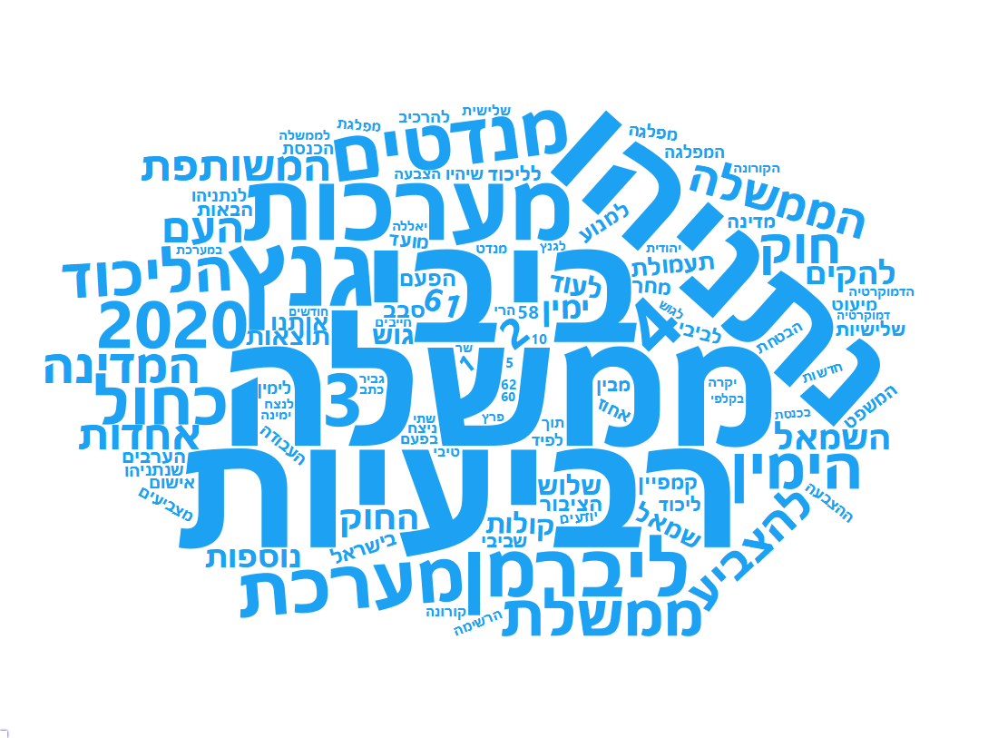
Figure 1: Wordcloud excludes Hebrew stop words and the word ‘elections’
What we can see is many of the words we’d expect: Political candidates, government, fourth (in the context of fourth elections), partis’ names and more. I’ll provide a more thorough discussion following our bigram plot below, as I believe it addresses many of the same words.
Common Bigrams
Like we did before, we can break up our text data into two word observations, also known as bigrams. In order to account for all combinations, we break up the sentence to fit all possible options. For example, assume we have the following sentence:
“Danny went to vote yesterday”
Using the unnest_tokens we’ll break the sentence into the following bigrams:
- Danny went
- went to
- to vote
- vote yesterday
Which gives us all possible options. We will also include two columns consisting of the bigram broken up into single words. This will help in filtering out bigrams containing Hebrew stop words or English words. I’ll not run through the following code but instead will point you to David Ronbinson & Julia Silge ‘Text Mining with R’ Book for further reading.
elec_bigram <- elections %>%
  select(text) %>%
  unnest_tokens(bigram, text, token = "ngrams", n = 2) %>%
  separate(bigram, into = c("word1", "word2"), sep = " ", remove = FALSE) %>%
  filter(!word1 %in% he_stopwords$word,
         !word2 %in% he_stopwords$word,
         !grepl("([a-z]+|בחירות)", bigram)) %>%
  count(word1, word2, sort = T) %>%
  slice(1:45) %>%
  graph_from_data_frame()

p_arrow <- arrow(type = "closed", length = unit(.1, "inches"))

ggraph(elec_bigram, layout = "fr")+
  geom_edge_link(aes(edge_alpha = n), arrow = p_arrow, end_cap = circle(.04, "inches"), show.legend = FALSE)+
  geom_node_point(color = "lightblue", size = 3)+
  geom_node_text(aes(label = name), vjust = 1, hjust = 1, family = "Calibri")+
  theme_void()+
  labs(title = "Twitter text bigram")+
  theme(text = element_text(family = "Calibri"),
        plot.title = element_text(hjust = 0.5 , face = "bold", size = 18))
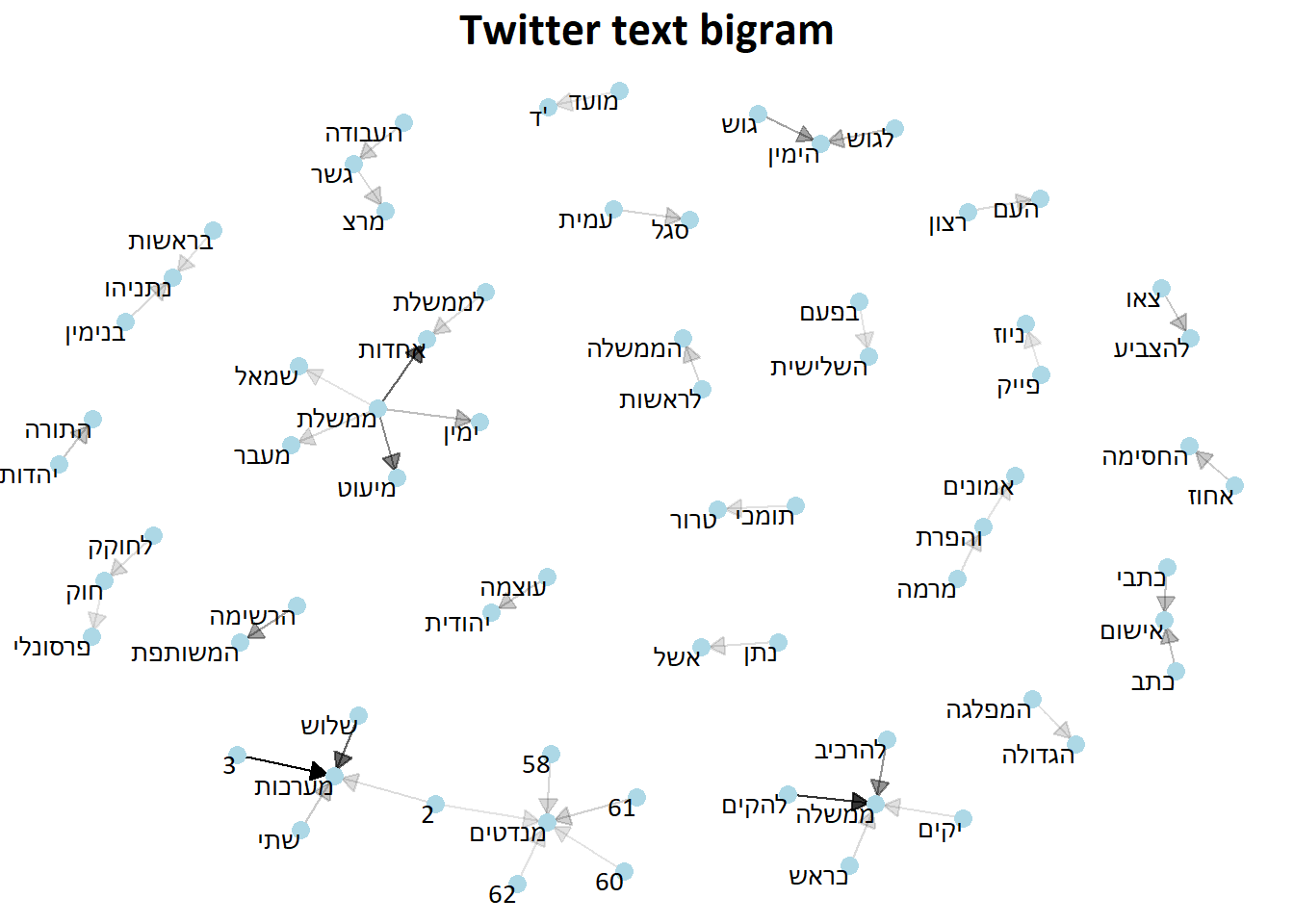
Figure 2: Word bigram excludes Hebrew stop words and the word ‘elections’
How should we read this graph?
First off, We only plotted the 45 most common bigrams (out of 100,000+). Every word is connected to another word with an arrow pointing to a given direction. The direction to which the arrow points is the way to read that bigram. In addition, bolder lines represent a higher frequency of that bigram throughout all our text.
For example, on the bottom of our graph we see the number ‘2’ connected to the words ‘mandates’ and ‘campagin’. The direction of the arrow signals that we should read the bigram as ‘2 mandates’ and ‘2 campagins’.
What does this all mean?
-
We have discussions regarding the number of chairs a govenrment will have (62/61/60/58) connected to mentions of the number of election campaigns (2/3) we had, discussions of a united and/or minimal government and the forming of one in general.
-
We see mentions of individuals such as “Benjamin Netanyahu”, “Amit Segal” (Both we discussed earlier), “Natan Eshel”, but no mention of the main candidate running against Netanyahu - “Benny Gantz”. That’s actually kind of odd, but more on that in a minute.
-
We also see mentions of political parties such as “Meretz”, “Gesher” and “Labor” who ran together this time around, “Otzma Yehudit”, “United Torah Judaism”, and the “Joint List”. There’s no mention of the two leading parties - “Kahol Lavan” & “The Likkud”., despite the mentioning of the latter’s leader.
-
Mentions of Netanyahu’s indicment and the personal law associated him.
-
Mentions I’d categorize as ‘other’ such as “Terrorist supporters”, “Will of the people”, “Fake news”, “Go vote’, etc.
Actaully, this turned out more interesting than I thought. Several questions arose while looking at it: Several words are missing such as the main parties names (Likkud & Kahol-Lavan), The leading oponent running against Benjamin Netanyahu - Benny Gantz - and other questions such as with whom are specific terms associated. Before we close up I’ll look at one question that troubles me - Why doesn’t Gantz appear in our list 😱?
Benny Gantz’s disappearance
In order to see why Benny Gantz doesn’t appear in our bigram plot I’ll do the following: I’ll break the text into bigrams and filter to have only the bigrams containing the word Gantz. Once we have that we can see why he doesn’t appear in our bigram plot despite appearing in our wordcloud.
Before I run the analysis and give you the answer think for a moment - What was the process of coming up with the bigram? If I chose only the 50 most frequent bigrams, why would a word that appears many times in our text not appear in our bigram list? Alternatively, did we filter anything along the way? Maybe even give the previous chunk another glance before I answer it.
Let’s have a look:
gantz <-elections %>%
  select(text) %>%
  unnest_tokens(bigram, text, token = "ngrams", n = 2) %>%
  separate(bigram, into = c("word1", "word2"), sep = " ", remove = FALSE) %>%
  filter(word1 %in% "גנץ" |
         word2 %in% "גנץ",
         !grepl("([a-z]+|בחירות)", bigram))
The code is similar to what we did earlier only this time we left bigrams that match the word we want - bigrams containing the word Gantz. Now that we have our list of bigrams, let’s look at the count of bigrams containing the word גנץ (‘Gantz’):
gantz %>%
  count(bigram, sort = T)
## # A tibble: 955 x 2
##    bigram         n
##    <chr>      <int>
##  1 של גנץ       160
##  2 בני גנץ      138
##  3 גנץ לא        90
##  4 על גנץ        70
##  5 את גנץ        69
##  6 עם גנץ        61
##  7 אם גנץ        41
##  8 גנץ היה       25
##  9 גנץ או        19
## 10 גנץ ליברמן    19
## # ... with 945 more rows
AHA! Now I see what happened. The first bigram is a stop word and the word Gantz (‘Of Gantz’). The second bigram should have been included as it is Gantz’s full name - Benny Gantz, which appears 138 times.
So, why has it been filtered? This is a great question which we can answer if we look at our stop words we initially used. Let’s see if it has the word בני (‘benny’ in Hebrew):
he_stopwords %>%
  filter(word == "בני")
## # A tibble: 1 x 1
##   word
##   <chr>
## 1 בני
Yes it does. At the time of writing this blog post it leaves me in a dilemma - Should I change the stop words file I used to a different one or maybe create my own? Or should I continue as is? I think leaving it will teach me (and hopefully whoever read this far) a valuable lesson of always checking your stop words. In a different context the specific bigram wouldn’t have got me thinking, but here it didn’t make sense that our leading candidate was filtered, thus my inquire into what happened. In hebrew the word Benny also means ‘my son’, which I wouldn’t describe as a stop word but whoever made the dataset I guess did.
If you wish to give it a try yourself, you can find the data in the form of an .rds or smaller .csv (excludes list columns) in my
github repository.
Well then, that’s all for now folks! And remember, make sure to validate your stop words dataset!
- Posted on:
- April 20, 2020
- Length:
- 15 minute read, 3014 words
- Categories:
- R
- See Also:
- Learning Tfidf with Political Theorists